slope distance D = 150 m measured at a slope of 12°. Find the horizontal distance.

 slope distance D = 150 m measured at a slope of 12°. Find the horizontal distance.

Solution:

Step 1: Horizontal distance formula

$$H = D \cos \theta$$ $$H = 150 \cos 12° \approx 150 \cdot 0.9781 \approx 146.7 m$$

✅ Answer: Horizontal distance = 146.7 m

You are given a closed traverse with four sides, three of its interior angles A, B and D are given. Find out the bearings of the four lines if the bearing of the line AB is given.

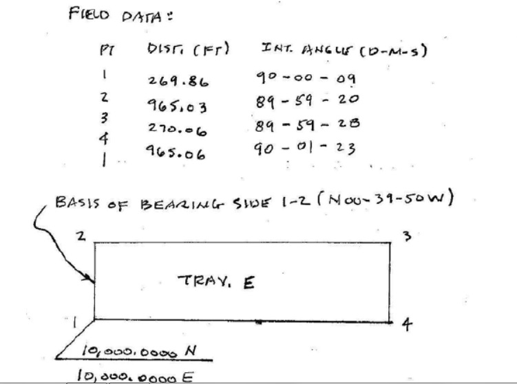
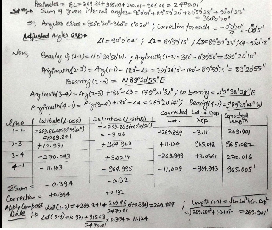
 You are given a closed traverse with four sides, three of its interior angles A, B and D are given. Find out the bearings of the four lines if the bearing of the line AB is given.

Solutions:

closed traverse- Compass survey - finding out Bearings of lines.

Following is the Field Data for a 4 sided, closed traverse, and you have to find the azimuth, bearings and corrected distances using Compass Rule or Bowditch Method.

 Problem:

Following is the Field Data for a 4 sided, closed traverse, and you have to find the azimuth, bearings and corrected distances using Compass Rule or Bowditch Method.

Solution: 

what equipments are used in Differential leveling?

 Differential leveling?

Equipment

The equipment list for differential leveling minimally includes:

• Level instrument
• Tripod
• Level rod

Although not always needed, a rod bubble and turning pin or turtle are often included.

a. Level Instrument

A level instrument is a telescope mounted so that it can be oriented horizontally.

(1) Traditional

Traditional levels are four-screw instruments. This refers to the four screws at the leveling head which are used to level the instrument. These levels typically have a long telescope and a bubble vial with a high sensitivity bubble. The higher the bubble sensitivity, the more quickly it reacts to level screw adjustment. A sensitive bubble is necessary to accurately establish a horizontal LoS. Four-screw instruments are either a Dumpy or Wye type.

A Dumpy level, Figure B-4, is the simpler of the two. Its telescope and bubble vial are rigidly attached to the upper part of the instrument. This upper part can be rotated horizontally and has a lock and slow motion for fine pointing.

Figure B-4 Dumpy Level

One or both ends of the bubble vial have screws or nuts allowing the ABT to be adjusted.

A Wye level is similar to a Dumpy except the telescope, including the bubble tube, is clamped in a pair of Y-shaped saddles (wyes), Figure B-5.

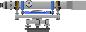Figure B-5  Wye Level

When the clamps are opened, the telescope and bubble can be removed, Figure B-6.

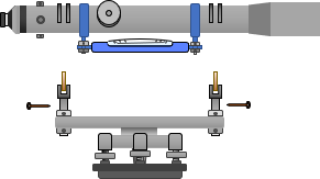Figure B-6 Opened Wye Level

The telescope can be turned end for end and replaced. This capability is not used while running a level circuit. So what is it for? It is primarily used as another way to check and adjust the instrument.

Of the two, the Dumpy level was more common and produced up through the 1980s.

All four leveling screws must be snugly in contact with the leveling head or the instrument will wobble. During instrument leveling, diagonal screws are turned opposite each other to center the bubble. Screws are easily under- or over-tightened. An under-tightened screw will cause the instrument to rock on the leveling head. Over-tightening will make the screw motions stiff and possibly warp the leveling head.

Because the bubble is so sensitive, slight screw rotations can cause considerable bubble movement. The surveyor can waste time "chasing the bubble" and use a single screw for minor adjustment, which in turn, contributes to under- and over-tightening.

These contribute to make instrument setup frustrating for the novice surveyor. While initially challenging, setup becomes easier and more efficient with practice.

(2) Automatic 

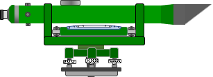
The most common modern instrument is an Automatic level, Figure B-7.

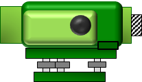Figure B-7 Automatic Level

It is a three-screw instrument making it impossible for the instrument to wobble like a four-screw instrument can.

The automatic level gets its name from an internal compensation system which automatically maintains a horizontal LoS if the instrument is disturbed. The compensation system uses a combination of fixed and free swinging prisms and mirrors. When the instrument is tilted the compensation system reacts to maintain a horizontal sight line at the observer’s end. The stylized cross-sectional views in Figure B-8 shows how the incoming horizontal LoS is reflected and refracted and emerges at the eyepiece in a parallel path.

Figure B-8 Compensator Reacting

 

The instrument is leveled using a circular bubble. The etched circle on the bubble glass is a general indicator of the compensator's operating range. If the bubble is outside the circle, the compensator may be at its physical limit and unable to maintain a horizontal LoS.

b. Tripod

A tripod is a three-legged support platform for the level, Figure B-9. The tripod's primary material can be wood, metal, fiberglass, or plastic; its legs fixed length or extendable. It usually has a flat top and a mounting screw for instrument attachment. The tripod’s function is to ensure a stable instrument setup for reliable measurements.

Figure B-9 Tripod

c. Level Rod

A level rod is a tall linear measuring scale. In English units, the divisions may be feet and decimal feet or feet-inches and fractional inches. Feet and decimal feet are most commonly used. In the metric system the divisions are meters and decimal meters.

The rod can be constructed of wood, metal, or fiberglass. Most rods telescope or extend in order to allow large elevation difference determinations yet collapse into a compact form.

There are many width and gradation styles depending on application. The most universal design is the Philadelphia rod, a portion of which is shown in Figure B-10.

	Red numbers are the full foot readings. Black numbers are the 0.1 ft readings The bars are each 0.01 ft tall and spaced 0.01 ft apart. Peaks on the bars correspond to the adjacent 0.1 or foot reading. A peak without an adjacent number corresponds to a half-tenth or 0.05 ft. At distances up to about 300 feet, a Philadelphia rod can be read directly to 0.01 ft.
Figure B-10 Level Rod

 Reading a rod consists of identifying the full foot and tenth foot, then counting up or down to determine the hundredth foot.

Figure B-11 shows some example rod readings.

Figure B-11 Example Rod Readings

 

The reading must be made with the rod held vertically to correctly determine instrument height above a point. There are a few ways to ensure the rod is vertical when the reading is made.

One method is to use a rod bubble, Figure B-12. This is a circular bubble which is held against or mounted to a level rod. The rod is vertical when the bubble is centered.

Figure B-12 Rod Bubble

 

 If a rod bubble is not available, then the rod can be waved, or rocked, slowly back and forth, Figure B-13.

The instrument operator will see the rod reading increase and decrease as the rod is waved. The reading is too high when the rod is tilted forward or backward. It is lowest when the rod is vertical. The operator records that reading. 

Figure B-13 Waving the Rod

 

 d. Turning point

Often when running a level line the distances between points may be too long for reliable reading or there may be obstructions. In such cases intermediate temporary points are established and leveled through. If a suitable stable point is not available then a turning point is used.

A turning point is usually a steel pin with a rounded top which can be firmly pounded into the ground, Figure B-14. It is left in position until after a BS reading is taken on it and the next elevation point established. Only then is it safe to remove the pin since its elevation is no longer needed.

Where the surface is hard, making it difficult to pound in a pin, a turtle can be used instead. A turtle is a heavy triangular or circular steel plate with three short equally spaced legs and a short rounded pin at top center, Figure B-15. When placed, the weight of the turtle helps keep it relatively stable while readings are taken. On some surfaces, dropping the turtle helps seat its legs more firmly providing additional stability.

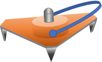Figure B-14 Turning Point		Figure B-15 Turtle

 

whar are the principles of Differential leveling?

 Differential leveling

 Principle

Differential leveling uses the vertical distance difference between two points to transfer an elevation from one point to another.

A summary of the process:

A Level is setup between two points, one whose elevation is known, Figure B-1.

Figure B-1 Setting Up

 

A backsight (BS) reading is taken on the known point, Figure B-2, using a rod divided into feet (or meters) and subdivisions thereof. This determines how far above the LoS is above the known point. Adding the BS reading to the point elevation gives the elevation of the instrument (EI, aka, Height of the Instrument, HI).

Figure B-2 Backsight Reading

 

A foresight (FS) reading is taken on the unknown point, Figure B-3, to determine how far above it the LoS is. Subtracting the FS reading from the instrument elevation gives the point elevation.

Figure B-3 Foresight Reading

 

The elevation of B is determined by adding the difference between the BS and FS readings:

ElevB = ElevRed+(BSRed-FSB)

The instrument is moved to a position between B and the next point and the process repeated.

Determine the elevation of B.M. 2 from the following notes. Check arithmetic by adding F.S.s and B.S.s. Sta. B.S. H.I. F.S. Elevation B.M. 1 1.21 50.00 T.P. 1 6.20 4.65 T.P. 2 4.82 3.11 T.P. 3 3.03 5.22 B.M. 2 3.16

 Problem 

Determine the elevation of B.M. 2 from the following notes. Check arithmetic by adding F.S.s and B.S.s.

Sta.	B.S.	H.I.	F.S.	Elevation
B.M. 1	1.21			50.00
T.P. 1	6.20		4.65
T.P. 2	4.82		3.11
T.P. 3	3.03		5.22
B.M. 2			3.16

Solution  

Sta.	B.S.	H.I.	F.S.	Elevation
B.M. 1	1.21			50.00
		51.21
T.P.1	6.20		4.65	46.56
		52.76
T.P. 2	4.82		3.11	49.65
		54.47
T.P. 3	3.03		5.22	49.65
		52.28
B.M. 2			3.16	49.12
Sum	15.26		16.14

OR

Sta.	B.S.	H.I.	F.S.	Elevation
B.M. 1	1.21	51.21		50.00
T.P.1	6.20	52.76	4.65	46.56
T.P. 2	4.82	54.47	3.11	49.65
T.P. 3	3.03	52.28	5.22	49.65
B.M. 2			3.16	49.12
Sum	15.26		16.14

Sum (B.S.) - Sum (F.S.) = 15.26 - 16.14 = -0.88

Elev B.M. 2 - Elev B.M. 1 = 49.12 - 50.00 = -0.88

Arithmetic check: do these differences equal?

Sum (B.S.) - Sum (F.S.) = Elev B.M. 2 - Elev B.M. 1

Answer: yes, they do equal

From the survey in Fig. 3.16, check the arithmetic by summing the B.S. and the F.S. Hint: Select only F.S. applicable to the differential survey. What is the error? Sta. B.S. H.I. F.S. Elevation B.M.1 4.38 100.00 104.38 0 + 00 3.04 101.34 0 + 50 2.81 101.57 1 + 00 5.43 98.95 1 + 50 6.12 98.26 2 + 00 2.15 4.11 100.27 102.42 2 + 50 7.16 95.26 3 + 00 5.01 97.41 3 + 50 7.15 1.29 101.13 108.28 4 + 00 2.16 106.12 4 + 10 1.19 107.09 B.M. 1 8.30 99.98

 Problem 

From the survey in Fig. 3.16, check the arithmetic by summing the B.S. and the F.S. Hint: Select only F.S. applicable to the differential survey. What is the error?

Sta.	B.S.	H.I.	F.S.	Elevation
B.M.1	4.38			100.00
		104.38
0 + 00			3.04	101.34
0 + 50			2.81	101.57
1 + 00			5.43	98.95
1 + 50			6.12	98.26
2 + 00	2.15		4.11	100.27
		102.42
2 + 50			7.16	95.26
3 + 00			5.01	97.41
3 + 50	7.15		1.29	101.13
		108.28
4 + 00			2.16	106.12
4 + 10			1.19	107.09
B.M. 1			8.30	99.98

Solution 

Sta.	B.S.	H.I.	F.S.	Elevation
B.M.1	4.38			100.00
		104.38
0 + 00			3.04	101.34
0 + 50			2.81	101.57
1 + 00			5.43	98.95
1 + 50			6.12	98.26
2 + 00 (T.P. 1)	2.15		4.11	100.27
		102.42
2 + 50			7.16	95.26
3 + 00			5.01	97.41
3 + 50 (T.P. 2)	7.15		1.29	101.13
		108.28
4 + 00			2.16	106.12
4 + 10			1.19	107.09
B.M. 1			8.30	99.98
Sum	13.68		13.70

Sum (B.S.) - Sum (F.S.) = 13.68 - 13.70 = -0.02

Elev B.M. 1(calc) - Elev B.M. 1(given) = 99.98 - 100.00 = -0.02

Math check: Sum (B.S.) - Sum (F.S.) = Elev B.M. 1(calc) - Elev B.M. 1(given)

differences are equal, therefore the math checks.

Accuracy of the work = error = Elev B.M. 1(given) - Elev B.M. 1(calc) = 100.00 - 99.98 = 0.02

Allowable error = 0.007[length of traverse, ft/100]**1/2 length of traverse, ft = 4 + 10 = 410 ft (from figure 3.16 field notes)

Allowable error = (0.007)[410 ft/100]**1/2 = 0.014

Therefore, the survey is not within reasonable accuracy because calculated error exceeds allowable error.

Compound Curves with examples (surveying)

 Compound Curves

a. Geometry

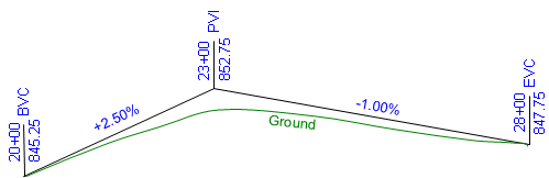
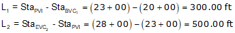
Sometimes a simple equal tangent vertical curve cannot be fit to a particular design condition. For example, the vertical curve in Figure B-24 must start at an existing intersection at sta 20+00 elev 845.25 ft and end at a second intersection at sta 28+00 elev 847.75 ft. To minimize earthwork an incoming grade of +2.50% is followed by an outgoing grade of -1.00%. This places the PVI at sta 23+00 elev 852.75 ft.

Figure B-24 Fitting a Curve

 

This combination results in a PVI that is not midway between the BVC and EVC. If a 600.00 ft equal tangent curve were used, it would begin at 20+00 and end at 26+00, 200.00 ft back along the -1.00% grade from the specified EVC.

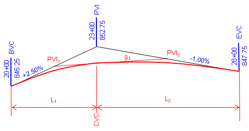
This situation requires an unequal tangent vertical curve. While a mathematical curve other than a parabolic arc could be used, the traditional method is to use two back-to-back equal tangent curves. This is referred to as a compound curve, Figure B-25.

Figure B-25 Compound Curve

 

A compound curve isn't as complex as it looks: the key is to break it into two successive equal tangent veritical curves.

PVIs are created for each curve at midpoint on the grade lines. A new grade, g3, is created by connecting the new PVIs. This is the outgoing grade for the first curve and the incoming grade for the second.

The CVC is the Curve to Vertical Curve point which is the EVC of the first curve and the BVC of the second; its station is the same as the overall PVI station. Once we have sufficient information for each curve to set up its Curve Equation, we can compute each curve independently.

The closer the individual curve's k values, the smoother the transition between them, particularly when there is a large grade change over a short distance.

b. Curve Equation

For an equal tangent vertical curve, we set up and solved Equations B-4 and B-5 through B-7. When setting these up for the curves in a compound curve, care must be taken to use the correct grades and lengths in each. Using subscripts i and m for the first and second curves respectively, their equations are:

	Curve 1	Curve 2
Equation B-5
Equation B-7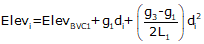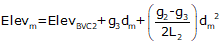
Equation B-8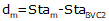
Equation B-9

 

c. High/Low Point

A compound curve has the same high/low point condition as an equal tangent curve: it occurs where the curve grade passes through 0%.

For the compound curve shown in Figure B-24: the first curve has two positive grades so it never tops out, the second begins with a positive and ends with a negative grade. That places the highest point of this compound curve on the second curve.

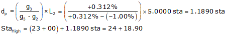
When using the equation to compute distance to the low/high point, remember:

• use the grades for the curve on which the point occurs, and,
• the distance computed is from the BVC of the curve on which the point occurs.

For example, the distance equation Equation B-8 is:

Equation B-10

 

Setting up Equation B-10 and hi/low point station for each curve:

	Distance	Station
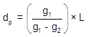
Curve 1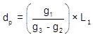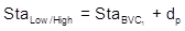
Curve 2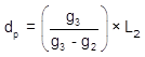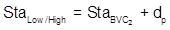

 

Remember: the high/low point occurs only on one curve or the other. Should g3 be 0%, then the low/high point would be at the CVC. If all three grades are positive or negative, then Equation B-10 does not apply as neither curve tops/bottoms out.

Example

Using the data given in Figure B-25:

(1) Complete the following table below
(2) Setup the Curve Equations for both curves
(3) Determine the station and elevation of the highest curve point.

Sketch

(1) Complete the table

Curve 1	Component	Curve 2
	incoming grade (%)
	outgoing grade (%)
	Length (ft)
	BVC Sta
	BVC Elev
	PVI Sta
	PVI Elev
	EVC Sta
	EVC Elev

 

Entries that can be made from the given criteria:

Curve 1	Component	Curve 2
+2.50	incoming grade (%)
	outgoing grade (%)	-1.00
	Length (ft)
20+00	BVC Sta	23+00
845.25	BVC Elev
	PVI Sta
	PVI Elev
23+00	EVC Sta	28+00
	EVC Elev	847.75

 

Compute:

 

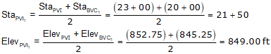
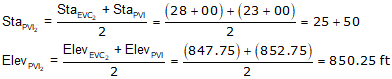
Since the PVIs are halfway along the grade lines, their positions are the averages of the grade line ends.

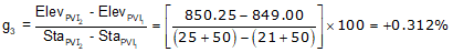
g3 is the grade of the line connecting the two curve PVIs. There can be different ways to compute it depending on the given data. In this example, we can use the position of the PVIs.

Compute the CVC elevation from PVI1.

The CVC elevation can also be computed from PVI2. We'll do it as a math check.

Complete the table.

Curve 1	Component	Curve 2
+2.50	incoming grade (%)	+0.312
+0.312	outgoing grade (%)	-1.00
300.00	Length (ft)	500.00
20+00	BVC Sta	23+00
845.25	BVC Elev	849.47
21+50	PVI Sta	25+50
849.00	PVI Elev	850.25
23+00	EVC Sta	28+00
849.47	EVC Elev	847.75

 

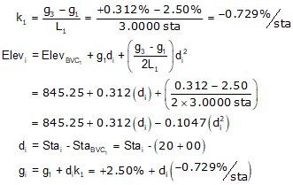
(2) Set up curve equations

Curve 1

Curve 2

Once these are set up, a Curve Table can be computed for each curve.

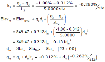
(3) Station and elevation of highest curve point.

The highest point will occur on Curve 2 since its grades go through 0%.

Use the equations for Curve 2.